Table of contents
Open Table of contents
Introduction
Quite often when coding up civil engineering problems there has been some level of an optimization problem.
In some cases the optimization is quite straightforward. For example for a steel truss in tension at 50% utilisation we could reduce the section area by half to get a utilisation of 100% therefore fully optimizing the amount of steel that we have used in our design. The linear relation means optimization is quite straightforward and we don’t need a particularly complex algorithm to find the solution.
In other cases there might be a parabolic relation. Such a problem would be called convex minimization problem. In this case we might use some iterative approach to converge on a solution, since we know that in this case if we find a local minimum value it is also the global minimum value.
However in some applications like slope stability analysis we might converge on a local minimum value that is not the global minimum value. This is called a non-convex minimization problem. In this case we might need to use some sort of algorithm to find the global minimum value.
In this post I primarily want to discuss non-convex minimization problems and heuristic algorithms that can be used to solve them. I will introduce some python code that helps illustrate how these algorithms can be applied and we can together evaluate their performance.
Basics of Optimization
Minimization vs Maximization
In optimization problems we are often trying to minimize a function. However, in some cases we might be trying to maximize a function. In this case we can simply multiply the function by -1 and then minimize it.
Hence we generally talk about minimization when referring to optimization problems, with it implied that such a solution could also be used to maximize a function.
Local vs Global Minima
A local minima is a point in the function where the function value is lower than all of its neighbors. It looks like the bottom of a valley.
A global minima is a the local minima with the lowest function value. It is the deepest valley with respect to the entire function.
We are generally interested in only finding the global minima.
Approaches to Optimizations
Optimization problems can be tackled in different ways depending on the nature of the function and the complexity of the problem. Broadly, these approaches can be divided into analytical methods and numerical methods.
Numerical methods are better suited for computers and include iterative and meta-heuristic methods.
Iterative Methods
Iterative solutions work well when dealing with convex optimization problems. Many different methods exist with common methods including:
- Gradient descent
- Newton’s method
Since this blog is more concerned with non-convex optimization problems I won’t go into detail about these methods. However, I will briefly go over an example to show why they wont work well for non-convex optimization problems.
These methods generally work off the assumption that there is only one minima in the function that can be converged upon by slowly moving down the slope of the function. This is a reasonable assumption for convex optimization problems, but not for non-convex optimization problems.
Both methods described require the derivative of the function to be calculated. This can be estimated for any function (since a mathematical relation is not always a given) using a finite differences approach.
The animation below shows the gradient descent method applied to the function f(x) = x^2. We converge on the global minimum value of 0.
The animation below shows the gradient descent method applied to the function f(x) = x^2 - cos(2πx) + 1. We converge on a local minima value and the result is sensitive to the starting point. We could get lucky and find the global minimum value of 0, but we could also get unlucky and find a local minima value of ~1. Once we are in a local minima we are stuck there and cannot escape.
Therefore we need some method that can escape from local minima and find the global minima in a time efficient manner.
Meta-Heuristic Algorithms
Meta-heuristic algorithms are especially useful when dealing with non-convex optimization problems, where the function we are trying to minimize might have many local minima. In such cases, classical methods like gradient descent can get stuck in one of those local valleys and fail to find the true global minimum.
Meta-heuristic methods work by exploring the search space more broadly, often using randomness, mimicry of natural processes, or population-based strategies. They are not guaranteed to find the perfect solution, but they often get very close—especially in complex, real-world scenarios like slope stability, where the failure surface might involve hundreds of variables and nonlinear interactions.
We could of course use more computationally expensive methods like to search every possible combination of variables to find the global minimum value. However, this is often not feasible in practice due to the sheer number of combinations and the time it would take to evaluate each one.
Common Meta-Heuristic Algorithms
The thing that first raised my attention to this topic was the interesting names behind these algorithms which are often inspired by nature. The cuckoo search algorithm for example mimics the way cuckoo birds lay their eggs in the nests of other birds. The cuckoo bird is a parasite and the algorithm mimics this behavior to find the best solution.
Other common algorithms include:
- Genetic Algorithm (GA)
- Particle Swarm Optimization (PSO): Mimics the social behavior of birds and fish, where individuals in a group adjust their positions based on their own experience and that of their neighbors.
- Ant Colony Optimization (ACO): Mimics the foraging behavior of ants, where they deposit pheromones to mark paths to food sources. The algorithm uses this information to find the shortest path to a solution.
- Simulated Annealing (SA): Mimics the annealing process in metallurgy, where materials are heated and then cooled to remove defects. The algorithm uses this process to explore the search space and find the best solution.
- Firefly Algorithm (FA): Mimics the flashing behavior of fireflies, where they attract mates and prey with their light. The algorithm uses this behavior to find the best solution.
- Bee Algorithm (BA): Mimics the foraging behavior of bees, where they communicate with each other to find the best food sources. The algorithm uses this behavior to find the best solution.
The remainder of this blog will be investigating the mechanisms behind these algorithms and how they can be applied to non-convex optimization problems. I will also be looking at the performance of these algorithms in terms of their ability to find the global minimum value.
In comparing these functions we will use the Rastrigin function.
Rastrigin Function
The Rastrigin function is a well-known test problem for optimization algorithms. It is a non-convex function used to evaluate the performance of optimization algorithms. It is very similar to the non-convex function shown earlier.
We now will also add an extra dimension to our function to make it a 3D function. The Rastrigin function is defined as the addition of a simple quadratic function and a periodic component. The function is defined as:
where:
- ( n ) is the number of dimensions (or variables)
- ( A ) is a constant (usually set to 10)
- ( x_i ) are the variables (or dimensions) of the function
- ( f ) is a constant that affects the periodicity of the cosine term (usually set to 1)
for a 2D function we would have:
if we break up the function into its components we can see that the function is made up of a simple quadratic function and a periodic component. The periodic component is what makes the function non-convex and gives it multiple local minima. The A variable controls the amplitude of the periodic component, that is the height of the peaks and valleys. The A*2 term shifts the minima so that the global minima is at (0,0) and has a value of 0.
For the illustrative example below I have set A=1.5 and f=2 for no reason other than it is easy to see in this visualization. In examples where we are looking to optimize the function we would set A=10 and f=1 and be searching within the bounds of -5.12 to 5.12.
Genetic Algorithm (GA)
The genetic algorithm mimics the process of natural selection, where the fittest individuals are selected for reproduction in order to produce the offspring of the next generation.
The idea is simple: You start with a random set of possible solutions (called a population), then apply genetic operators such as selection, crossover, and mutation to iteratively improve the solutions over several generations.
- Selection: Choose the best candidates.
- Crossover: Combine two candidates to create new ones.
- Mutation: Introduce random changes to maintain diversity.
This process repeats over multiple generations until the solution is close to optimal.
Genetic Algorithm for Rastrigin Function
For this function we are concerned with finding the optimal x and y values. We will give each candidate in our population an x and a y value (two genes) and the fitness of each candidate is calculated using the Rastrigin function.
Step 1: Initialize Population
In this step we create a random population of candidates. Each candidate is represented by a pair of x and y values. The number of candidates in the population is determined by the user.
# creates an array of random candidates with x y values in the range of -2 to 2
pop = np.random.uniform(LOWER_BOUND, UPPER_BOUND, (POP_SIZE, N_GENES))
Step 2: Evaluate Fitness
Next, we calculate the fitness of each candidate in the population. The fitness determines how “good” a solution is, guiding the selection of candidates for the next generation.
The fitness is calculated using the Rastrigin function (although the negative of the function is used since we are trying to minimize the function but the GA algorithm tries to maximize fitness).
# creates an array of fitness values for each candidate in the population
fit = -rastrigin(pop[:, 0], pop[:, 1])
Step 3: Selection
Once we have fitness values for all candidates, we need to select the best individuals to create the next generation. We use a simple tournament selection method, where two candidates are chosen at random, and the one with the better fitness (lower Rastrigin value) is selected.
def select(pop, fit):
    """
    Selects two candidates from the population using tournament selection.
    It randomly picks two individuals and selects the one with the best (lowest) fitness.
    """
    # Randomly select two individuals
    idx = np.random.randint(0, POP_SIZE, 2)
    # Return the one with better fitness
    return pop[idx[0]] if fit[idx[0]] > fit[idx[1]] else pop[idx[1]]
Step 4: Crossover
In this step, we combine the genetic information of two selected parents to create a new candidate solution (the child). The crossover is done uniformly, meaning each gene (X and Y) is chosen randomly from one of the two parents.
The crossover helps to combine the strengths of two good candidates to create a potentially better candidate.
def crossover(parent1, parent2):
    """
    Performs a uniform crossover between two parents to create a new individual (child).
    The crossover happens with a probability of 'CROSSOVER_RATE'. Each gene is randomly selected from one of the parents.
    """
    if np.random.rand() < CROSSOVER_RATE:
        # Generate a mask to randomly select genes from either parent
        mask = np.random.rand(N_GENES) > 0.5
        # Create a child by selecting genes from either parent based on the mask
        child = np.where(mask, parent1, parent2)
        return child
    else:
        # If no crossover happens, just return a copy of the first parent
        return parent1.copy()
Step 5: Mutation
Next, we introduce mutation to avoid the algorithm from getting stuck in a local minimum. Each individual in the population has a small chance of randomly changing one of its genes (either x or y).
def mutate(individual):
    """
    Performs mutation on an individual by modifying one of its genes.
    Each gene (X and Y) has a small probability of being changed.
    The mutation adds small Gaussian noise to the gene value, but ensures the new value stays within the bounds.
    """
    for i in range(N_GENES):
        # With probability 'MUTATION_RATE', apply a small mutation
        if np.random.rand() < MUTATION_RATE:
            individual[i] += np.random.normal(0, 0.1)  # Add Gaussian noise
            # Ensure the new value is within the specified bounds
            individual[i] = np.clip(individual[i], BOUNDS[0], BOUNDS[1])
    return individual
Step 6: Next Generation
Finally, we create the next generation of candidates by selecting parents, performing crossover, and applying mutation. This process is repeated for a specified number of generations.
Performance
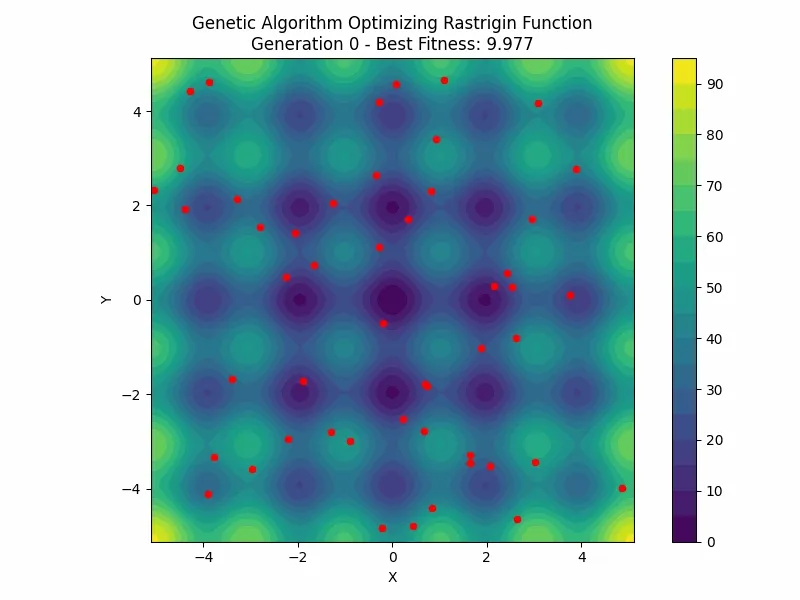
With an appropriate population size and number of generations the GA algorithm can find the global minimum value of the Rastrigin function quite well. However if the population size is too small or the number of generations is too low the algorithm can get stuck in a local minima.
Applying the GA algorithm to a specific problem might require some tuning of the parameters to get the best performance.
An animation of the algorithm with 50 candidates and 50 generations is shown below with a genetic mutation rate of 0.1 and a crossover rate of 0.9. The algorithm successfully converges on the global minimum value of 0.
Conclusion
Non-convex optimization problems are a common challenge in engineering and applied mathematics, where the presence of multiple local minima makes finding the global minimum difficult. Traditional iterative methods like gradient descent work well for convex problems but often fail in non-convex landscapes because they get trapped in local minima.
Meta-heuristic algorithms, such as Genetic Algorithms, Particle Swarm Optimization, and Simulated Annealing, offer practical solutions by exploring the search space more broadly and introducing randomness or population-based strategies. While they do not guarantee a perfect solution, they can effectively approximate the global minimum in complex problems, as demonstrated with the Rastrigin function and the Genetic Algorithm example.
The key takeaway is that understanding the nature of your optimization problem—convex or non-convex—guides the choice of method. For non-convex problems, leveraging meta-heuristic techniques can provide robust and computationally feasible solutions, opening the door to optimizing real-world systems that would otherwise be intractable.
Appendix - GA Full code
import numpy as np
import matplotlib.pyplot as plt
import matplotlib.animation as animation

# --- Define Rastrigin function ---
def rastrigin(X, Y):
    A = 10
    return A * 2 + (X**2 - A * np.cos(1 * np.pi * X)) + (Y**2 - A * np.cos(1 * np.pi * Y))

# --- GA parameters ---
POP_SIZE = 50
N_GENERATIONS = 30
MUTATION_RATE = 0.1
CROSSOVER_RATE = 0.9
LOWER_BOUND = -5.12
UPPER_BOUND = 5.12
N_GENES = 2

def initialize_population():
    """
    Initializes a random population of solutions within the given bounds.
    The population consists of 'POP_SIZE' individuals, and each individual has 'N_GENES' (X and Y).
    """
    return np.random.uniform(LOWER_BOUND, UPPER_BOUND, (POP_SIZE, N_GENES))

# --- Fitness function ---
def fitness(pop):
    """
    Calculates the fitness of each individual in the population.
    Since we're minimizing the Rastrigin function, we use the negative value of the function
    as the fitness score (lower Rastrigin value means better fitness).
    """
    return -rastrigin(pop[:, 0], pop[:, 1])

# --- Selection (Tournament) ---
def select(pop, fit):
    """
    Selects two candidates from the population using tournament selection.
    It randomly picks two individuals and selects the one with the best (lowest) fitness.
    """
    # Randomly select two individuals
    idx = np.random.randint(0, POP_SIZE, 2)
    # Return the one with better fitness
    return pop[idx[0]] if fit[idx[0]] > fit[idx[1]] else pop[idx[1]]

# --- Crossover (Uniform) ---
def crossover(parent1, parent2):
    """
    Performs a uniform crossover between two parents to create a new individual (child).
    The crossover happens with a probability of 'CROSSOVER_RATE'. Each gene is randomly selected from one of the parents.
    """
    if np.random.rand() < CROSSOVER_RATE:
        # Generate a mask to randomly select genes from either parent
        mask = np.random.rand(N_GENES) > 0.5
        # Create a child by selecting genes from either parent based on the mask
        child = np.where(mask, parent1, parent2)
        return child
    else:
        # If no crossover happens, just return a copy of the first parent
        return parent1.copy()

# --- Mutation ---
def mutate(individual):
    """
    Performs mutation on an individual by modifying one of its genes.
    Each gene (X and Y) has a small probability of being changed.
    The mutation adds small Gaussian noise to the gene value, but ensures the new value stays within the bounds.
    """
    for i in range(N_GENES):
        # With probability 'MUTATION_RATE', apply a small mutation
        if np.random.rand() < MUTATION_RATE:
            individual[i] += np.random.normal(0, 0.1)  # Add Gaussian noise
            # Ensure the new value is within the specified bounds
            individual[i] = np.clip(individual[i], LOWER_BOUND, UPPER_BOUND)
    return individual

# --- Main GA Loop (Collect populations for animation) ---
def genetic_algorithm():
    """
    The core loop of the genetic algorithm. This function iterates through generations,
    performing selection, crossover, and mutation at each step to evolve the population.
    The population history is stored to track the evolution.
    """
    pop = initialize_population()  # Initialize the population randomly
    history = [pop.copy()]  # Store the initial population in history

    # Iterate for a predefined number of generations
    for _ in range(N_GENERATIONS):
        fit = fitness(pop)  # Evaluate the fitness of the population
        new_pop = []  # Create a new population

        # Generate the new population by selecting parents, applying crossover and mutation
        for _ in range(POP_SIZE):
            parent1 = select(pop, fit)  # Select the first parent
            parent2 = select(pop, fit)  # Select the second parent
            child = crossover(parent1, parent2)  # Crossover the parents
            child = mutate(child)  # Mutate the child
            new_pop.append(child)  # Add the child to the new population

        # Replace the old population with the new one
        pop = np.array(new_pop)
        history.append(pop.copy())  # Store the new population in history for animation

    return history  # Return the history of the population over all generations

# --- Run GA ---
populations = genetic_algorithm()

# --- Set up figure ---
x = np.linspace(LOWER_BOUND, UPPER_BOUND, 1000)
y = np.linspace(LOWER_BOUND, UPPER_BOUND, 1000)
X, Y = np.meshgrid(x, y)
Z = rastrigin(X, Y)

fig, ax = plt.subplots(figsize=(8, 6))
contour = ax.contourf(X, Y, Z, levels=20, cmap='viridis', linewidths=1.5)

# Add colorbar (works as a "legend" for the contour colors)
cbar = fig.colorbar(contour)
# cbar.set_label('Fitness Value')

# Create the scatter plot (GA population)
# scat = ax.scatter([], [], color='red', s=20, label='Population')
scat = ax.scatter([], [], color='red', s=20)

# Set axis labels and title
ax.set_xlim(LOWER_BOUND, UPPER_BOUND)
ax.set_ylim(LOWER_BOUND, UPPER_BOUND)
ax.set_xlabel('X')
ax.set_ylabel('Y')
ax.set_aspect('equal')

# Add a legend for the red points
# ax.legend(loc='upper right')

# --- Animation update function ---
def update(frame):
    pop = populations[frame]
    scat.set_offsets(pop)
    best_fitness = np.max(fitness(pop))  # Find best fitness in current generation
    ax.set_title(f"Genetic Algorithm Optimizing Rastrigin Function\n"
                 f"Generation {frame} - Best Fitness: {(-best_fitness):.3f}")
    return scat,

# --- Animate ---
ani = animation.FuncAnimation(fig, update, frames=len(populations),
                               interval=100, blit=True)

plt.tight_layout()
plt.show()

# Optionally save:
ani.save('ga_rastrigin.gif', writer='pillow', fps=5)
# ani.save('ga_rastrigin.mp4', writer='ffmpeg', fps=10)